|
Prediction the Workability of High-Performance Concrete using neural network An example of a multivariate regression problem using Neuroph by Marija Selakovic, Faculty of Organizational Sciences, University of Belgrade an experiment for Intelligent Systems course
Introduction The function regression problem can be regarded as the problem of approximating a function from noisy or corrupted data. Here the neural network learns from knowledge represented by a training data set consisting of input-target examples. The targets are a specification of what the response to the inputs should be. The basic goal in a function regression problem is to model the conditional distribution of the output variables, conditioned on the input variables. In this experiment it will be shown how neural networks and Neuroph Studio are used when it comes to problems of regression. Several architectures will be tried out, and it will be determined which ones represent a good solution to the problem, and which ones do not.
Introduction to the problem Nowadays, mix design of high-performance concrete is more complicated because involves many variables and includes various mineral and chemical admixtures. To date, the construction industry had to depend on a relatively few human experts to give recommendations in solving high performance concrete mix design problem. This would normally require expensive human expert. However the situation may be improved with the use of artificial intelligence that manipulates the human brain in the way of thinking and giving suggestion.. The usefulness of artificial intelligence in solving difficult problems has become recognized and their development is being pursued in many fields. Applications of Artificial Neural Network in high performance concrete mix design is discussed in the form of modeling its strength and workability requirement together with many different additive materials. The aim of this experiment is to train neural network for predicting slump, flow and 28-day compressive strength in High-Performance Concrete. The data contained a total 106 results of these test. Using the data, neural networks are trained for the input:
Prodecure of training a neural network In order to train a neural network, there are six steps to be made: 1. Normalize the data 2. Create a Neuroph project 3. Create a training set 4. Create a neural network 5. Train the network 6. Test the network to make sure that it is trained properly
Step 1. Data Normalization Data normalization is the final preprocessing step. In normalizing data, the goal is to ensure that the statistical distribution of values for each net input and output is roughly uniform. In addition, the values should be scaled to match the range of the input neurons. The typically range is from 0 to 1. This means that along with any other transformations performed on network inputs, each input should be normalized as well. The formula for normalizing the data is:
Where: X - value that should be normalizedXn - normalized value Xmin - minimum value of X Xmax - maximum value of X
Step 2. Creating a new Neuroph project To create Neuroph Project click File > New Project
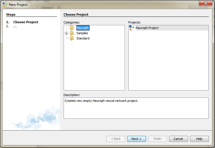
Select Neuroph Project, and click Next.
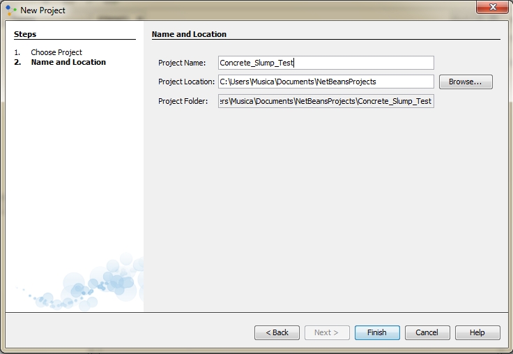
Enter project name and location and click Finish.
This will create the new Neuroph Project.
Step 3. Create a Training Set When training multilayer networks, the general practice is to first divide the data into three subsets. The first subset is the training set, which is used for computing the gradient and updating the network weights and biases. The second subset is the validation set. The error on the validation set is monitored during the training process. The validation error normally decreases during the initial phase of training, as does the training set error. However, when the network begins to overfit the data, the error on the validation set typically begins to rise. The network weights and biases are saved at the minimum of the validation set error. The test set error is not used during training, but it is used to compare different models. It is also useful to plot the test set error during the training process. If the error on the test set reaches a minimum at a significantly different iteration number than the validation set error, this might indicate a poor division of the data set. In order to this, dataset will be divided into three groups. First will consist 70% of all data for training purpose, second 20% for validation, and 10% for testing. Now, we are ready to create new training set. To create training set do the foolowing: Click File > New File to open training set wizard:
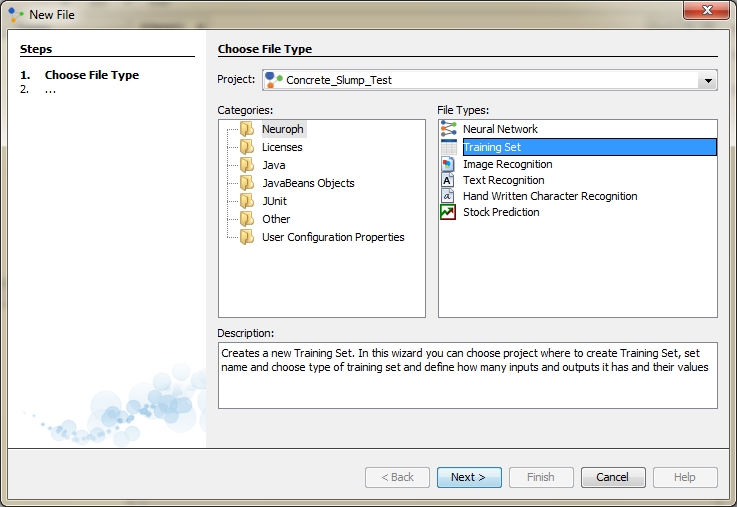
Select training set file type, then click next:
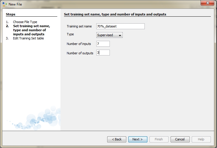
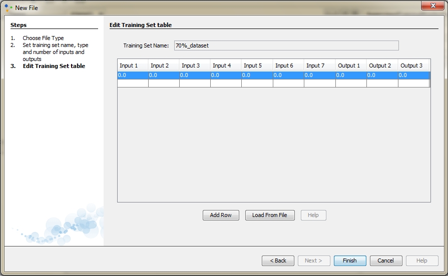
Enter training set name and select the type of supervised. Supervised training is accomplished by giving the neural network a set of sample data along with the anticipated outputs from each of these samples. Supervised training is the most common form of neural network training. As supervised training proceeds, the neural network is taken through several iterations, or epochs, until the actual output of the neural network matches the anticipated output, with a reasonably small error. Each epoch is one pass through the training samples. Unsupervised training is similar to supervised training except that no anticipated outputs are provided. Unsupervised training usually occurs when the neural network is to classify the inputs into several groups. Therefore we choose supervised learning. In field Number of inputs enter 7 and in field number of outputs enter 3 and click next:
Then you can create set in two ways. You can either create training set by entering elements as input and desired output values of neurons in input and output label, or you can create training set by choosing an option load file. The first method of data entry is time consuming, and there is also a risk to make a mistake when entering data. Therefore, choose second way and click load from file.
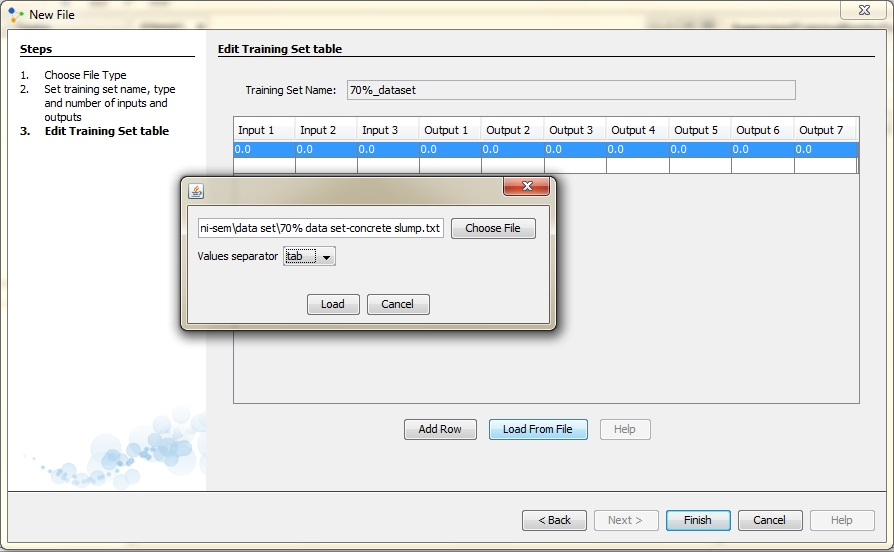
Click on Choose File and find file named 70% dataset-concrete slump.txt. Then select a separator. In our case values have been separated with tab. When you finish this, click on Load.
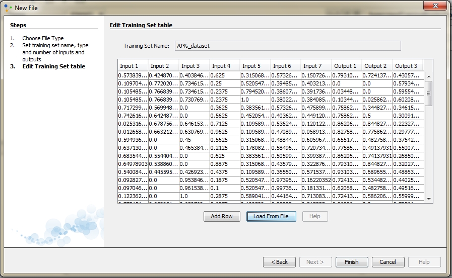
A new window will appear and table to the window is our training set. We can see that this table has a total of 10 columns which is fine because the 7 columns represents input values and other 3 columns represents output values. We can also see that all data are in the certain range, range between 0 and 1. Click Finish and new training set will appear in the Projects window. In same way we will create other two subsets.
Step 4.1 Create a Neural Network In order to make a network able to solve more complex problems, we will choose the Multi-Layer Perceptron (MLP) type which is one of the most widely applied and researched Artificial Neural Network model. MLP networks are normally applied to performing supervised learning tasks, which involve iterative training methods to adjust the connection weights within the network. This is commonly formulated as a multivariate non-linear optimization problem over a very high-dimensional space of possible weight configurations. Create Multi Layer Perceptron network Click File > New File
Select desired project from Project drop-down menu, Neuroph as category, Neural Network file type and click next.
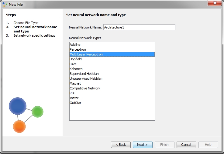
Enter network name, select Multi Layer Perceptron, click next.
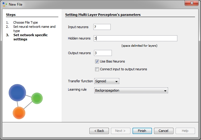
In new Multi Layer Perceptron dialog enter number of neurons. The number of input features corresponds to the number of input neurons in the neural network, while the number of test types usually corresponds to the output neurons. In this example, since we have three different tests, we are using three output neuron. We also need to set the number of hidden neurons (and layers), which depends on the classification complexity. Hidden neurons are neurons between the input and output layer, and MLP networks may have one or more hidden layers. Though these layers do not directly interact with the external environment, they have a tremendous influence on the final output. Both the number of hidden layers and the number of neurons in each of these hidden layers must be carefully considered. Using too few neurons in the hidden layers will result in something called underfitting. Underfitting occurs when there are too few neurons in the hidden layers to adequately detect the signals in a complicated data set. Using too many neurons in the hidden layers can result in several problems. First, too many neurons in the hidden layers may result in overfitting. Overfitting occurs when the neural network has so much information processing capacity that the limited amount of information contained in the training set is not enough to train all of the neurons in the hidden layers. A second problem can occur even when the training data is sufficient. An inordinately large number of neurons in the hidden layers can increase the time it takes to train the network. The amount of training time can increase to the point that it is impossible to adequately train the neural network. Obviously, some compromise must be reached between too many and too few neurons in the hidden layers. In the corresponding field, enter the number of neurons that are in the hidden layers. Separate the numbers with a space. For this, we will try with 3 neurons Furthermore, we check option Use Bias Neuron. Bias neurons are added to neural networks to help them learn patterns. A bias neuron is nothing more than a neuron that has a constant output of 1. Because the bias neurons have a constant output of one they are not connected to the previous layer.If values in the data set are in the interval between -1 and 1, choose Tanh transfer function. In our data set, values are in the interval between 0 and 1, so we used Sigmoid transfer function. As learning rule choose Backpropagation With Momentum. Backpropagation With Momentum algorithm shows a much higher rate of convergence than the Backpropagation algorithm. On the end click Finish.
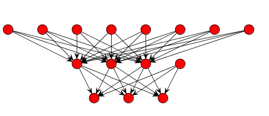
Appearance of the neural network, we just created, you can see in the figure bellow. Just select Graph View.
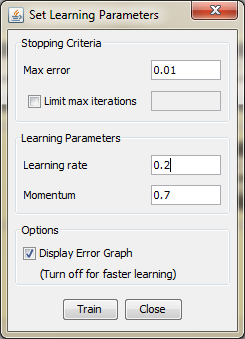
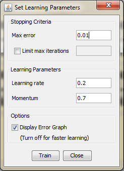
The network diagram shown above is a full-connected, three layer, feed-forward, perceptron neural network. "Fully connected" means that the output from each input and hidden neuron is distributed to all of the neurons in the following layer. "Feed forward" means that the values only move from input to hidden to output layers; no values are fed back to earlier layers. Step 5.1 Train the network To start network training procedure, in network window select training set from drop down list and click Train button.Next thing we should do is determine the values of learning parameters, learning rate and momentum, and max error. the learning rate - the selection of a learning rate is of critical importance in finding the true global minimum of the error distance.Backpropagation training with too small a learning rate will make agonizingly slow progress. Too large a learning rate will proceed much faster, but may simply produce oscillations between relatively poor solutions. momentum - empirical evidence shows that the use of a term called momentum in the backpropagation algorithm can be helpful in speeding the convergence and avoiding local minima. The idea about using a momentum is to stabilize the weight change by making nonradical revisions using a combination of the gradient decreasing term with a fraction of the previous weight change. The hope is that the momentum will allow a larger learning rate and that this will speed convergence and avoid local minima. On the other hand, a learning rate of 1 with no momentum will be much faster when no problem with local minima or non-convergence is encountered The maximum error will be 0.01, and learning rate 0.2 and momentum will be 0.7
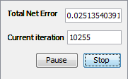
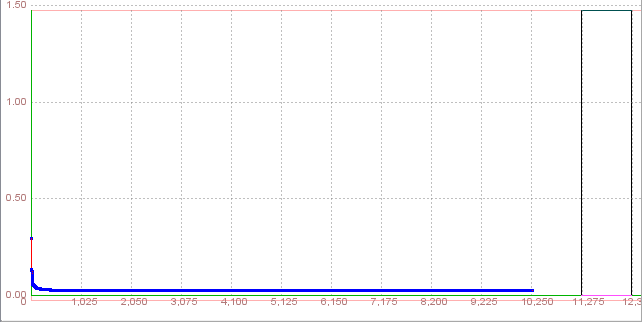
Now, click Train button. This will start training and open network learning graph and iteration counter, so we can obesrve the learning process Training was unsuccessfully, total net error was higher than permissible
In the beginning of training total net error fluctuated, followed by constant and slight rise. Training wasn't completed after 10255 iterations, so we can not test the network.
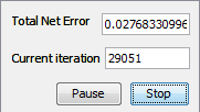
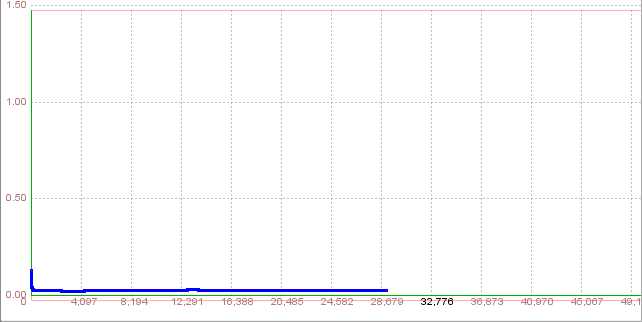
Training attempt 2Step 5.2. Train the network In order to accomplish error less than 0.01 we will update the learning rate and momentum with increase to 0.3 and decrease to 0.5 respectively. In network window click Randomize button and then click Train button. Value of learning rate and momentum replace with a new value click Train button. During the training network with new parameters process of learning showed the similar trend. After 29051 iterations total error network was 0.027683 which was higher than upper limit.
The third attempt of training with learning parameters 0.5 and 0.7 respectively was also unsuccessful. Total net error was approximately 0.03 after 27552 iterations. It is clear that increase the value of learning rate lead to rise and total net error. The table below illustrates the results of all (three) trainings for the architecture with three hidden neurons. Table 1. Training results for the first architecture
Based on information from Table 1 it can be observed that the difference between obtained total net error and expected upper limit for this error is actually small. Because of that, we should add a few hidden neurons in following attempts. As a consequence, this error will be smaller.
Step 4.6. Create a Neural Network In previous section there was too few neurons in the hidden layers. As a result, they couldn't adequately detect the signals in complicated data set. For this, we put more emphasis on studying appropriate architecture an learning parameters. As we can see in earlier attempts total net error increased with rise of learning rate. For this reason, learning rate will remain on low level. For training we will use the same data set, which consist 70% of full data set. It is necessary to select the same options as in the previous architecures, instead of the number of hidden neurons, which will be 5 in this attempt. Step 5.6. Train the network Regarding the former section we put for learning rate 0.2 and for momentum 0.7. For field set Stoping criteria we put 0.01 as max error.
After entering this values click on button Train and the training process starts.
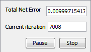
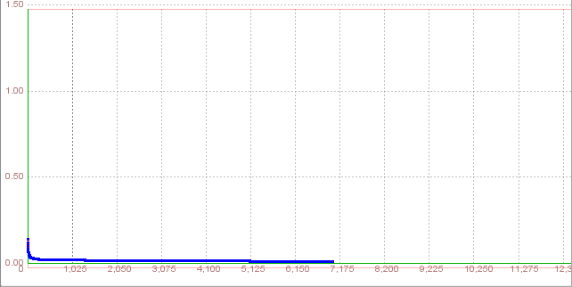
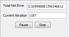
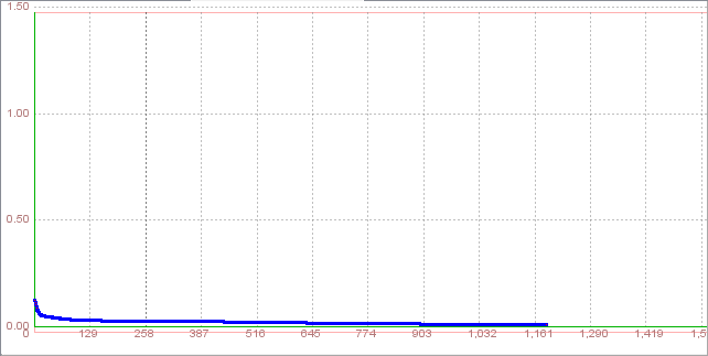
After 7008 iterations Total Net Error drop down to a specified level of 0.01 which means that training process was successful
ValidationOnce a neural network has been trained it must be evaluated to see if it is ready for actual use. This step is important so that it can be determined if additional training is required. To correctly validate a neural network, validation data must be set aside that is completely separate from the training data. In this case we use a 20% of full data set for validation.If the architecture is appropriate the validation process will be also successful with same parameters.
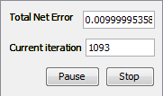
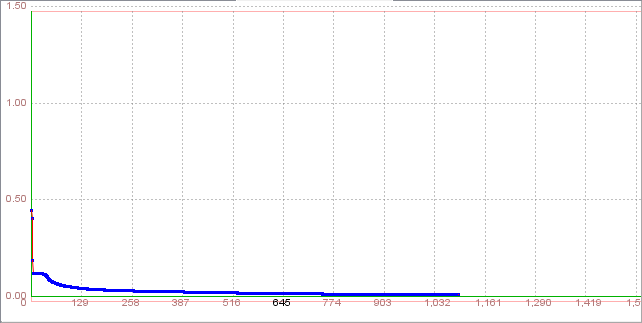
After 1093 iterations Total Net Error drop down to a specified level of 0.01 which means that validation was successful and we have to test this network. 6.6. Test the network The Testing set (in this case, 10% of full data set) is used to test the performance of a fully trained classifier. This is usually employed to determine the error rate of the final chosen model. For testing, we can click on 'Test' button and than we can see the testing results. It is noticable that Total Mean Square error is around 0.09.
The goal is to obtain a network with a high ability to generalize. This means that the error of the prediction of the test data has to be minimized. If the error of the output data during the training is small, but the error in the test-phase is large, the network does not generalize. So, we can conclude that that this type of this neural network architecture is not the best solution, and we should try some other.
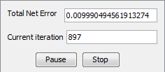
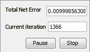
Step 5.7. Train the network Because of very high Total Mean Square error in previous training, we will try with other architecture. Instead of five hidden neurons neural network will be trained with six hidden neurons. Also, learning parameters, learning rate and momentum, will remain the same, as well as max error. As we expected, the training and validation process was sucessfu with same data sets. Training result
Validation result
Aslo a very important indicators, which is apparently from the graphs, is a similar numbers of iterations in training and validation process. Aslo the total net errors in this cases are very close, so that can indicate in a good generalization of network. 6.7. Test the network It is noticable form the results below that the Total Mean Square error is much lower than in former case. As we can see, there are few critical observation with big error in value of outputs. But, we will try with slight different architecture in order to improve this results.
Step 5.8. Train the network In this attempt we will try to get some better results by increasing the size of hidden neurons. It is known that number of hidden neurons is crucial for network training success, and now we will try with 7 hidden neurons. The summary of the results in training and validation process are shown below Training result Validation result
6.7. Test the network After testing a neural network, it is noticable that the total mean square error is approximately 0.0188 which is much lower than it was in previous attempts. As we can see, there are a few individual errors for output value, not too high compared with others. We use only 10% of full data set, and because of that, this can be a good result.
The tables below show the results in all trained network with described distribution of data set. This include also results in validation and testing. Table 2. Training and Validation results (total net error was same in both cases)
Table 3. Testing results (10% full data set)
From the tables above, we can see that the smallest total mean square error is accomplished by architecture with seven hidden neurons. On the other hand, we had a increase of this type of error with the change of architecture. If the error of the output data during the training is small, but the error in the test-phase is large, the network does not generalize. Often this means that we have to reduce the number of neurons in the hidden layer. But sometimes, the errors may have a different cause. For instance, we can not expect a small error in the output data, if the input data have a large statistical or systematic error.
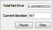
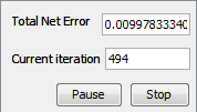
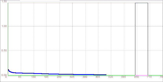
Step 4.10. Create a Neural Network During learning, the outputs of a supervised neural network come to approximate the target values given the inputs in the training set. This ability may be useful in itself, but more often the purpose of using a neural net is to generalize, to have the outputs of the net approximate target values given inputs that are not in the training set. But, generalizaton is not always possible. For creating the Neural Network model (yielding optimal performance) and to minimize the true error between actual and desired output, the data is randomly divided into three disjoint sets namely: Training set, Validation set, and Testing set. In earlier attempts, we used 70% of full data set for training, 20% for validation and 10% for testing. As we can saw the best result we get with neural network with seven hidden neurons. In next attempts, we will use the same architecture and learning parameters, but in order to accomplish the generalization of this network we will divide data set into new groups. In first case, we will use 40% of data set for training, and for both, validation and testing 30%.We will now train that network with the newly created training set, and observe whether the result will worsen. Step 5.10. Train the network We open the Network7, and select the 60% dataset-training, and then click 'Train'. The parameters that we now need to set will be the same as in previous attempts: the maximum error will be 0.01, the Learning rate 0.2, and the Momentum 0.7 We will not limit the maximum number of iterations, and we will check 'Display error graph', as we want the see how the error changes throughout the iteration sequence. After clicking 'Train', a window with the graph showing the function minimizing process will appear. We notice that the error stops at around 494th iteration.
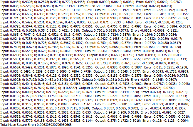
Validation process is done successfully with total net errorl lower than 0.01 and number of iteration, at 1048. Step 6.10. Test the network In previous testing we used only 10% of full data set, but now we use 30%, which consist more observations. After testing with this data we will choose randomly several observation in order to see individual errors and their contribution in total mean square error. Because of problem, network can estimate the results of slump and flow tests and strenght in High Performance Concrete.
The results are shown in the table above: the total mean square error is around 0.0063. We can conclude that this network has a good ability of generalization. Table 3. Individual errors
It is clear from table above that individual errors for each observation is slight higher than others. A majority of all outputs have error lower than 0.1. In conclusion, if you have a test case that is close to some training cases, the correct output for the test case will be close to the correct outputs for those training cases. If you have an adequate sample for your training set, every case in the population will be close to a sufficient number of training cases. Hence, under these conditions and with proper training, a neural network will be able to generalize reliably the workability of concrete. This will be also tried with other distribution of data set. In third case, we will divide all data on aslo three part. First consist 15% in purpose of validation, second 25% for testing and last one 60% data set for training. Comparation of these results and results gave in previous case is shown in table below. Table 4.Training and Validation results for other subsets:
Several different solutions tested in this experiment have shown that the choice of the number of hidden neurons is crucial to the effectiveness of a neural network. We have concluded that one layer of hidden neurons is enough in this case. Also, the experiment showed that the success of a neural network is very sensitive to parameters chosen in the training process. However, the learning rate must not be too high. Using a different proportion of data set for training, validation and testing we also shown the network ability in generalization. As the final selected and tuned Artificial Neural Network model has seven hidden neurons in one layer. During the testing and training, we found that Total Mean Square Error and Total Net Error were lower than 0.01. This proves clearly that the Neural Network models developed are reliable and useful, thus proving that splitting the data into three sets is quite effective for developing and selecting optimal Artificial Neural Network model and its final error estimation. In conclusion, Artificial Neural Networks can be used by engineers to estimate the slump, flow and strength in concrete whose constituents mainly includes cement, fly ash, flag, water, coarse aggregates, fine aggregates and super-plasticizer. It becomes convenient and easy to use these models to predict any result of these test (giving suitable mix proportions).
DOWNLOAD See also:
|
|||||||||||||||||||||||||||||||||||||||||||||||||||||||||||||||||||||||||||||||||||||||||||||||||||||||||||||||||||||||||||||||||||||||||||||||||||||||||||||||||||||||||||||||||||||||||||||||||||||||||||||||||||||||||||||||||||||||||||


